Pitfalls in trend analysis
UNDER CONSTRUCTION
Motivation
Trend analysis is one of the most important tools for estimating changes not only in economic but also in natural processes. In the debate about measures to mitigate the effects of climate change, precise knowledge of the current trend in temperature is essential.
Temperature data often show a very strong seasonality, so that trends are not only overlaid by natural random fluctuations but especially by seasonal fluctuations.
These considerations arose when considering the temperature data continuously collected at the time series station from 2007 to 2021 in the Spiekerooger back barrier.
The Problem
A time series can contain several trends, for example if a value temporarily rises or falls. In the broadest sense, this is also a seasonality but can also be superimposed on the “`real”’ seasonality.
What problems can arise if the requirements for a typical trend analysis are violated?. Can the trend be correctly predicted if the data shows strong seasonality? To answer this artificial data similar in their characteristics to natural data are examined.
The data
Artificial data similar to temperature data measured at the time series station within the East Frisian Wadden Sea for the years 2007-2017 are examined.
\(y(t)= 10 - 10 \cdot cos\left(\frac{2\pi(t-60)}{365}\right)+ 0.0001\cdot t\)
The data show the typical minimum end of February and are supposed to have a mean value and a seasonal amplitude of 10 °C.Time is supposed in units of days. A trend of 0.365 °C in 10 years is added. In this first step no noise is assumed.
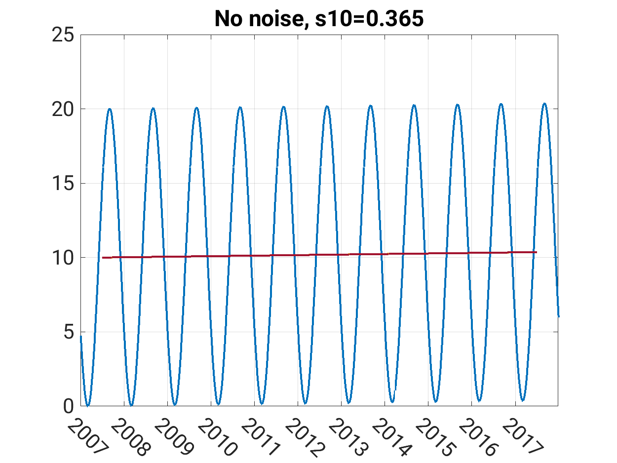
The blue line shows the data, the red line shows the assumed trend of 0.365 °C in ten years.
Methods
The methods are leant on Brockwell & Davis (2002). The trend of the daily data is estimated by the Theil-Sen-Estimator. The non-parametric Mann-Kendall-Test with a significance level of \(\alpha=0.05\) is used to decide if the data show a significant trend or not.
Naive solution
Taking eleven years of daily data as the basis for the trend analysis, the Theil-Sen estimator calculates a significant trend of 2.52 °C in 10 years.
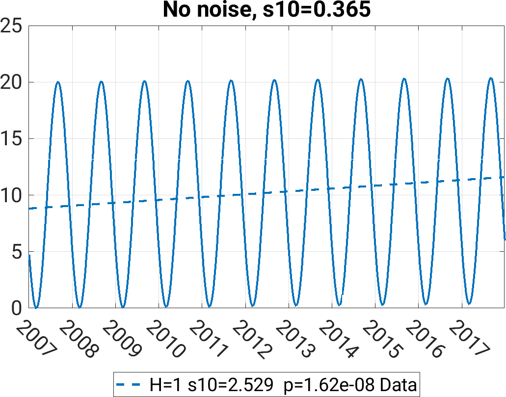
This result overestimates the real trend by far. Looking at the time series one can see that there is an intrinsic trend due to the start of the time series in January and ending in December. Thus, there is a asymmetric due to the sampling period. This becomes even clearer when the corresponding signal is analyzed without a trend. The Theil-Sen Estimator still outputs a trend of almost 2.16 °C over 10 years. Analyzing the trend-free signal from minimum to minimum or from maximum to maximum reveals no significant trend. The largest trend is achieved when the signal is sampled from inflection point to inflection point.
To improve this result, the signal must be processed before trend analysis. For this purpose, the signal is considered as a stochastic process consisting of a seasonal component, a trend component, and a noise component.
The stochastic process
The process is a superposition of a trend component, a seasonal component and an error term, also called a residual. The time base t is assumed to be discrete here.
\(x_t=m_t+s_t+e_t\)
Trend analysis is about estimating the trend component with the aim that \(m_t\) no longer contains any seasonal components. The remaining error process \(e_t\) should be a normal distributed homoscedastic stationary process1
Deseasonalization
Deseasonalization attempts to remove all seasonal components from the signal. This is often done by forming a running average or, more sophisticatedly, by calculating an average seasonality which can be substracted from the signal. For the given artifical data the variability of data without annual signal can be achieved by the following steps2:
- repeate first and last year
- calculate centered 365-days-running mean
- cut additional years
- subtract the running mean from the original
- calculate mean in every day of year over all years
- centering of result so that mean becomes zero*
- subtract result from the original data
The italicized steps are necessary to avoid errors at the beginning and at the end of the time series. The remaining process contains the trend component and the error terms.
One have to keep in mind that the assumption of a normal distributed homoscedastic stationary error is a requirement that is almost impossible to fulfill in reality. Consider signals that naturally have a lower bound at zero, such as irradiance data or nutrient concentrations. In this case, the seasonality and the characteristic of the error term will correlate.
UNDER CONSTRUCTION
Results
Data without noise
Running mean vs. running median
Conclusion
Footnotes
Stationary means that the statistical properties of the process, such as mean and variance, do not change over time. Scedasticity characterizes the error term. Homoscedastic error terms are distributed with constant variance, heteroscedastic error terms have some kind of pattern.↩︎
The used code is adapted from: https://de.mathworks.com/help/econ/seasonal-adjustment.html↩︎